The simulation

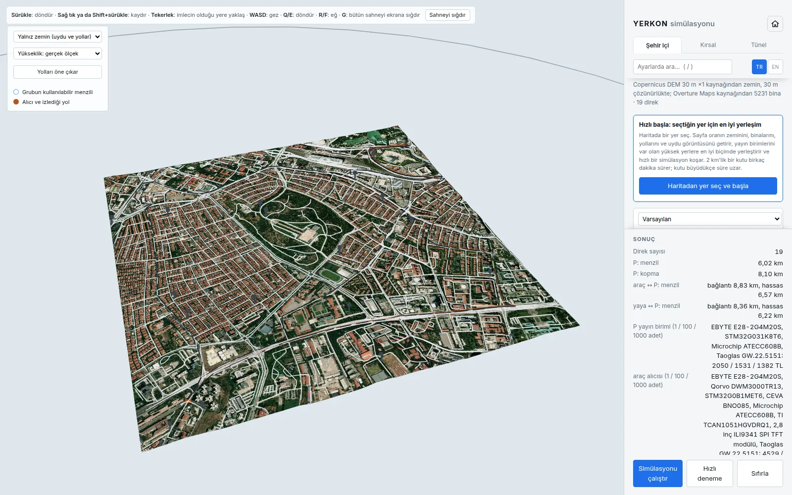
The ground is real

• All three rows stand on real ground near Ankara, fetched once from the Copernicus 30 m DEM and baked into the package, so a clone reproduces the table without touching the network.
• The city is Kızılay: three kilometres on a side, with 91 metres between its lowest and highest point. The open country is the Polatlı plain, twenty kilometres on a side with 486 metres of it. The tunnel is a real two kilometre bore through the mountains at Kızılcahamam.
• Nowhere is there a "flat ground" option. A flat surface is not the most neutral terrain the model can draw, it is the most favourable one: it would make the result look better than it is.

One calculation decides the range

• Nowhere in the code is there a number saying "the maximum range is this". Range comes out of working out how much the signal weakens on its way. The same calculation decides two things at once: whether the link holds, and how precisely it measures when it does.
• The signal reaches the receiver two ways: directly, and bouncing off the ground. Past a certain distance those two fall out of step and weaken each other. That distance grows with antenna height, so mounting a unit low costs range.
• The signal bends over obstacles and weakens doing it. The calculation looks at the whole terrain rather than the worst single obstacle on the path (ITU-R P.526-15 §4.5.2, delta Bullington). A link across Kızılay has three obstacles in front of it at the median, sixteen at the worst.
• The terrain is read every ten metres. Read at a fixed 64 points, a 6,9 km rural link would be read every 108 metres, and skipping the rises in between would put the loss at 31,28 dB where the answer is 37,60.
• A link counts the larger of those two losses, not their sum. Both describe what the same terrain does to the same link, and adding them would count the same hill twice.
• Shadowing sits on top of those: two links the same distance apart come out different depending on what stands between. 4 dB with a clear path, about 7,8 dB without (3GPP TR 38.901). It is random, so the calculation is repeated eight times and all the results of the eight are read together.

The messages and the position

• A distance is measured rather than calculated. Two radios send messages back and forth; on the SX1280 one ranging exchange takes 33,4 milliseconds, including the 5 % rest listen before talk (LBT) asks for.
• Measuring against twelve units in turn takes 401 milliseconds. A car doing 100 km/h covers 11,1 metres in that time, so the measurements in one round do not belong to one instant. The calculation does not pretend they do.
• The code that works out the position never sees where the vehicle really is. It sees only these: the measured distance, the unit's position as surveyed at installation, the time of the measurement, and how much that measurement is trusted.
• Units strung along a roadside are all at much the same height, which leaves the vertical hard to measure from ranges. The filter therefore takes the road's height from the receiver's map as a measurement, with a map error of 2,43 m drawn in patches along the road. The VPE column is the result.

Three errors that averaging will not remove

• A blocked link measures longer than it is. The signal goes around the obstacle and the measurement counts that longer way. The error always goes the same way, so measuring more often and averaging does not remove it.
• If a unit's position is surveyed wrong at installation, it stays wrong. It is drawn once per unit and carried to the end. In the tunnel the median error is 0,12 m with a perfect survey and about five times that with 15 cm of survey error. A position cannot be better than the survey of the units.
• A lost message gives no measurement. The 2,4 GHz band is shared with wireless networks, so it is crowded. 15% of messages are lost in the city, 5% on the open road, none in the tunnel.

What is left out

• The vehicle's motion sensor and wheel turns are left out. The filter combines only the radio measurements and the height from the map. The report's design has both, so these numbers are worse than a real vehicle's.
• The signal arriving by several paths after bouncing off building walls (multipath) is not modelled on its own; the model has the bounce off the ground and the long reading of a blocked link. The radio's own noise and the clock drifting during the exchange are in the model.
• The tunnel loss comes from a model measured in a real road tunnel at 2,8 to 5 GHz and carried to 6,5 GHz; it was not measured at 6,5 GHz.
• The security layer is absent too. Signature checking, key management and the "still working" messages the units send the centre belong to the design rather than to the simulation.

Places that are already high

In the urban and rural rows the anchors do not stand on a grid but where a placement search put them; the simulator's Find the best layout section and its Quick start box run the same search for another place picked on the map. The candidates are existing lighting columns and signs, poles along the road (lighting columns in town, electricity distribution poles in open country) and 25 m masts to be put up on hilltops. Roofs are rented from their owners, so they are not offered. Every candidate is tried with the link budget, and the choice is a cover search by lifecycle cost. A point counts as covered once four units reach it and they are spread over at least three of the four quarters around it. Units all strung along one street, on one side, cannot fix a position along that street.

The search finds the places and gives its own quick estimate; the simulation measures how accurate that placement really is. Apply the proposed layout and press Run the simulation to compare it with the layout it replaces on the same journey.

In the browser, and on your own machine

The Run the simulation button opens the simulator in this browser. No server computes anything: Python, numpy and this project's own package come down to the page and everything runs on this computer. The first load fetches about 20 MB and can take a minute; after that the browser keeps it. In a browser one processor does the work, so a run is slower than in a local install; Quick trial shortens it.

Republishing the table, fetching another city's ground, or running all three rows at full resolution needs a local install. Four commands:

The quick trial

The Quick trial button in the simulator and --fast on the command line coarsen the same two figures: the shadows are drawn once instead of pooled over eight, and the ground profile is read at a fixed 64 samples instead of every 10 m. A run drops from fifteen minutes to about one.

The coarse ground reads diffraction loss low, which mostly makes a fast answer flatter the deployment. The single shadow draw can err either way: on the same placement one row can come out better fast and another worse. A fast run is for trying things; the table on the Results page comes from the slow, full run only.

git clone https://github.com/ysoktar/yerkon
cd yerkon
pip install -e ".[dev]"
yerkon view